Data Analysis

Fandango

Fandango Media, LLC is an American ticketing company that sells movie tickets as well as give movies reviews. In 2015, Fandango faced allegations of providing misleading reviews for movies, as outlined in the mentioned article. FiveThirtyEight

Aim

When a company both displays, movie ratings and profits from selling tickets, there could be a bias toward higher ratings to boost sales. Transparency and audience awareness are essential to prevent such biases.The goal is to assess the data from Fandango and compare it with the claims made in the 538 article to ascertain whether Fandango's ratings in 2015 were indeed influenced to favor higher ratings, potentially to boost ticket sales.

Technologies Used

Language: python

Libraries: numpy, pandas, matplotlib and seaborn

Data

The data set is openly available on 538's github. There are two csv files, one with Fandango Stars and Displayed Ratings, and the other with aggregate data for movie ratings from other sites, like Metacritic, IMDB, and Rotten Tomatoes.

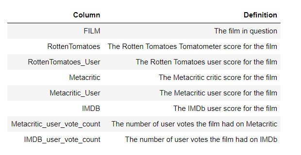
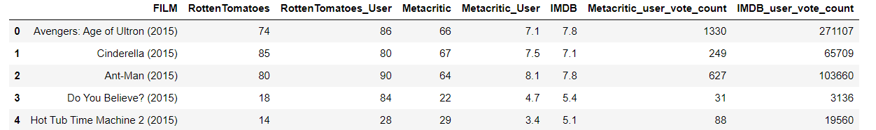
all_sites_scores.csv

all_sites_scores.csv contains every film that has a Rotten Tomatoes rating, a RT User rating, a Metacritic score, a Metacritic User score, and IMDb score, and at least 30 fan reviews on Fandango. The data from Fandango was pulled on Aug. 24, 2015.

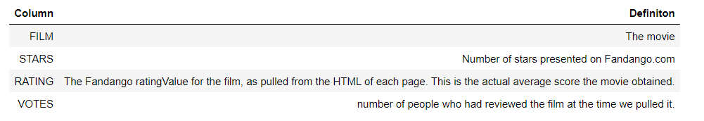
fandango_scape.csv

fandango_scrape.csv contains every film 538 pulled from Fandango.

part 1 :Fandango site

Importing


import numpy as np
import pandas as pd
import matplotlib.pyplot as plt
import seaborn as sns
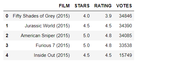
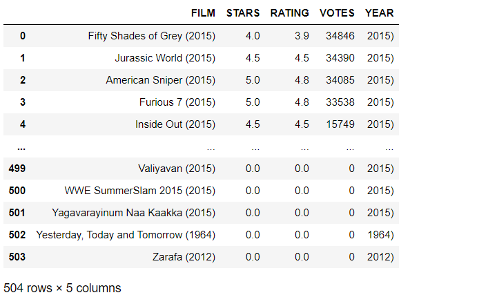
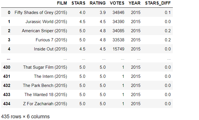
fandango = pd.read_csv("fandango_scrape.csv")
fandango.head()
    
                Output


       

        
            
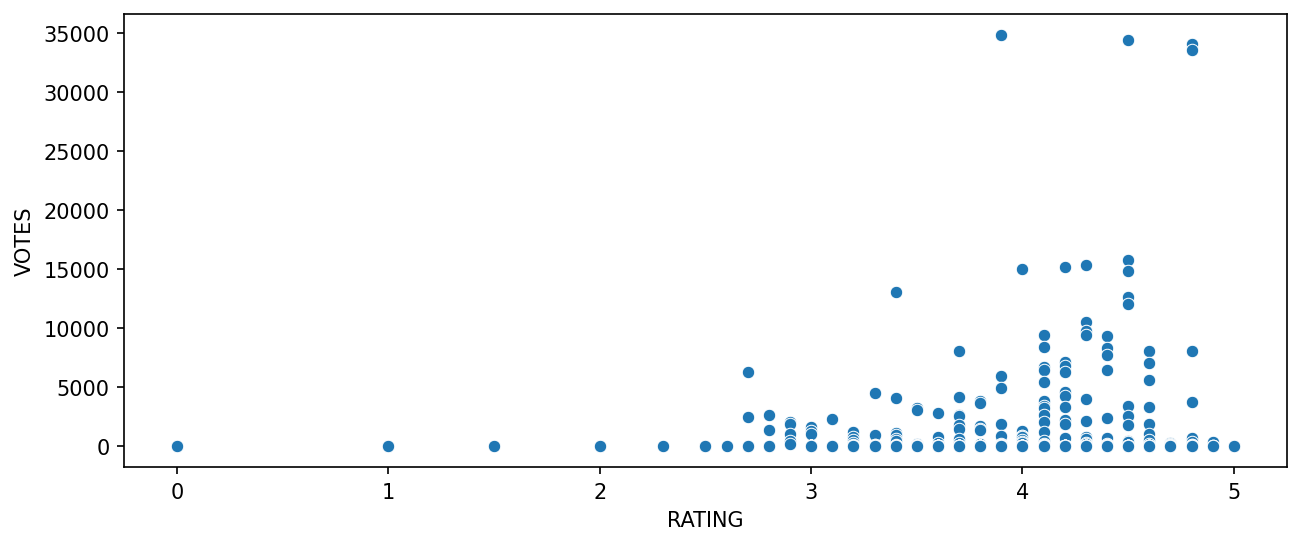
                The relationship between popularity of a film and its rating. By a scatterplot  which is showing the relationship between rating and votes.
                
plt.figure(figsize=(10,4),dpi=150)
sns.scatterplot(data=fandango,x='RATING',y='VOTES');
    
                Output
                

                    
           
        
        
               Creating a new column that is able to strip the year from the title strings and set this new column as YEAR
            
fandango['YEAR'] = fandango['FILM'].apply(lambda title:title.split('(')[-1]))
fandango

            Output
            
        
                
       
    



    
         number of movies in the Fandango DataFrame per year.
        
fandango['YEAR'].value_counts()


        Output
        
    
            
            

            
    
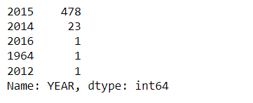
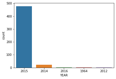
        The count of movies per year:
        
sns.countplot(data=fandango,x='YEAR')


        Output
        
            
            
 
            

            
    
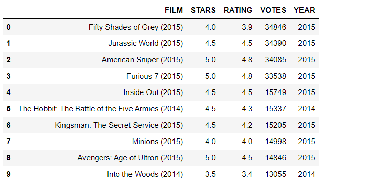
        the top 10 movies with the highest number of votes.
        
fandango.nlargest(10,'VOTES')

        Output
        
            
            
 
            

            
    
        removing any films that have zero votes.
        
fan_reviewed = fandango[fandango['VOTES']>0]


        
        
         
            
 
        

            
    
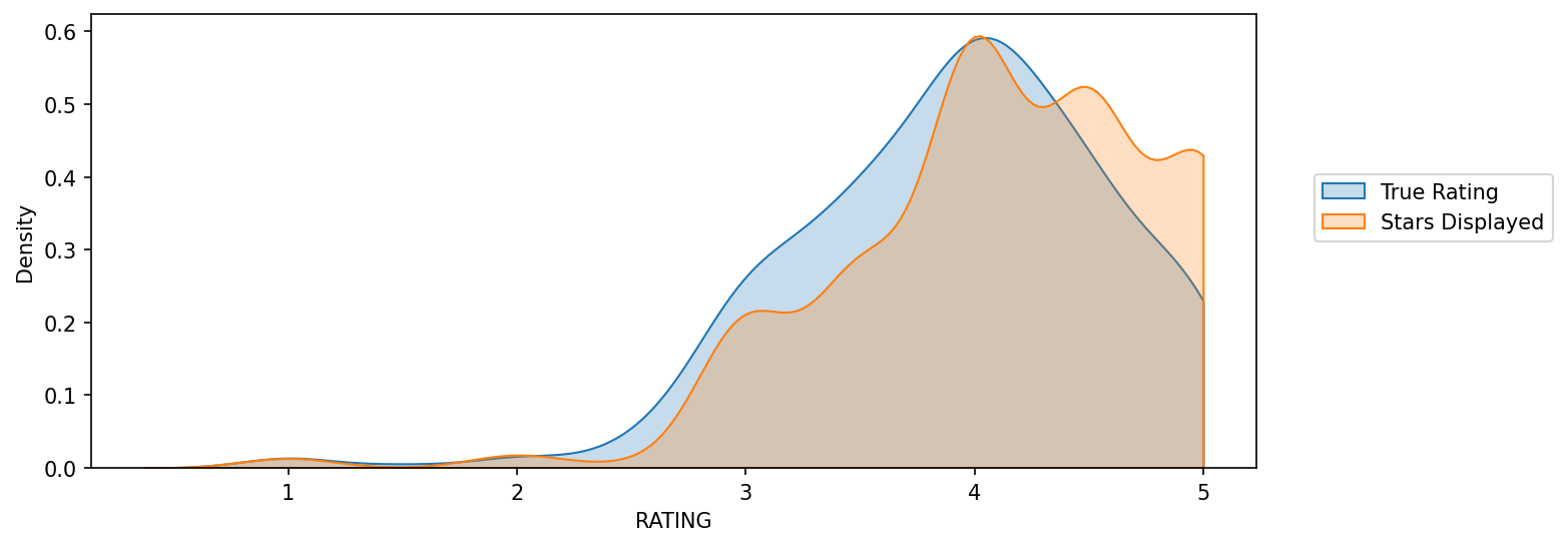
        KDE plot, that displays the distribution of ratings (STARS) versus what the true rating was from votes (RATING)
        
plt.figure(figsize=(10,4),dpi=150)
sns.kdeplot(data=fan_reviewed,x='RATING',clip=[0,5],fill=True,label='True Rating')
sns.kdeplot(data=fan_reviewed,x='STARS',clip=[0,5],fill=True,label='Stars Displayed')
            
plt.legend(loc=(1.05,0.5))


        Output
        

            
 
        

            
    
        Calculating this difference with STARS-RATING and rounding these differences to the nearest decimal point.
        
fan_reviewed["STARS_DIFF"] = fan_reviewed['STARS'] - fan_reviewed['RATING'] 
fan_reviewed['STARS_DIFF'] = fan_reviewed['STARS_DIFF'].round(2)
 fan_reviewed

        Output
        
        
            
        
            

            
    
         The count plot which display the number of times a certain difference occurs: 
        
plt.figure(figsize=(12,4),dpi=150)
sns.countplot(data=fan_reviewed,x='STARS_DIFF',palette='magma')


        Output
        
    
            
 
        

            
    
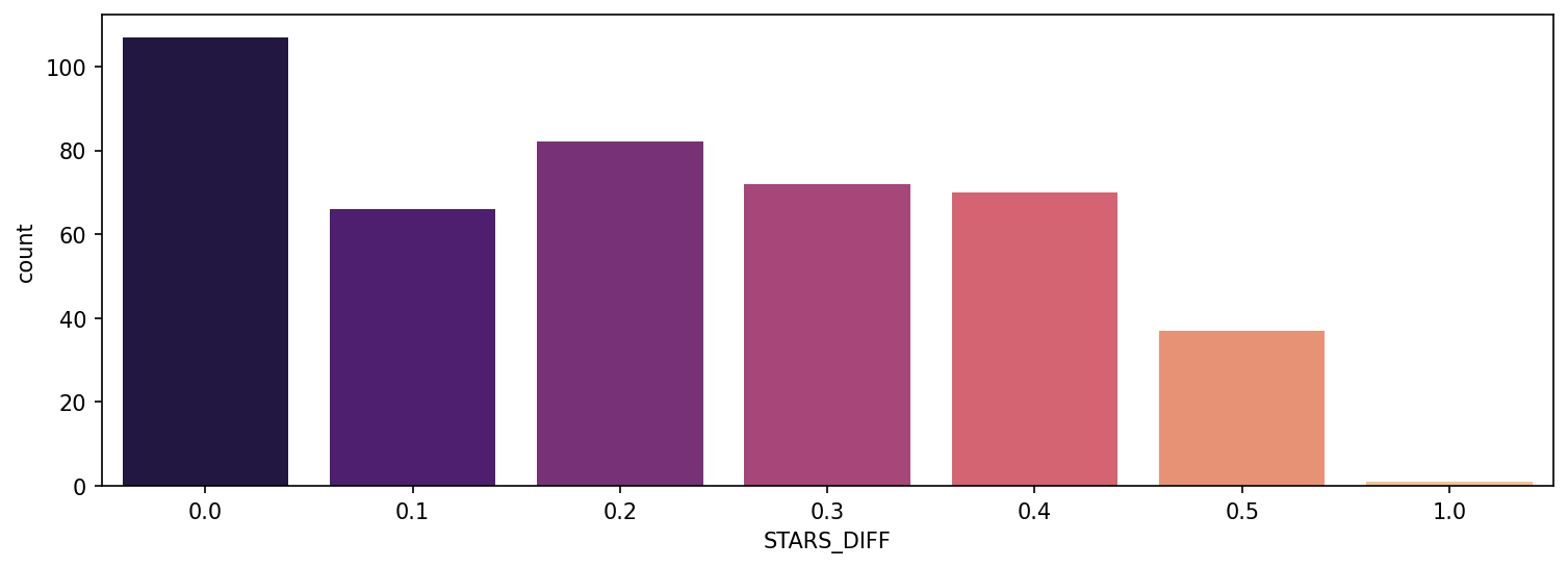
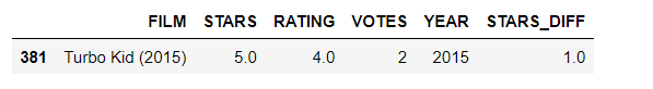
        the plot show that one movie was displaying over a 1 star difference than its true rating!
        
fan_reviewed[fan_reviewed['STARS_DIFF'] == 1]


        Output


     
         Part 2: Comparison of Fandango Ratings to Other Sites  
            
                
                
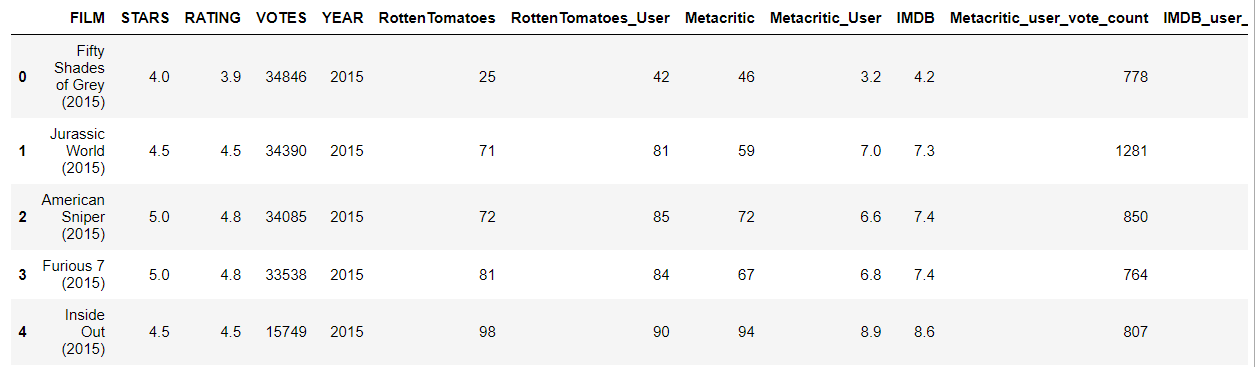
all_sites = pd.read_csv("all_sites_scores.csv")        
all_sites.head()       
        
                Output
                

                    
         

         
            
            
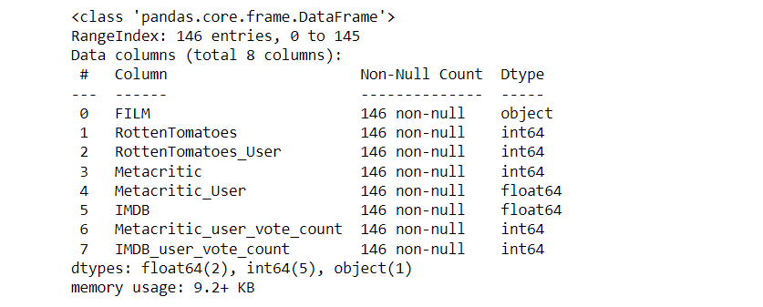
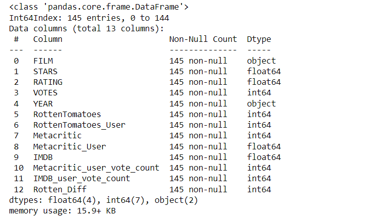
all_sites.info()   
    
            Output
            
                
                
     




     
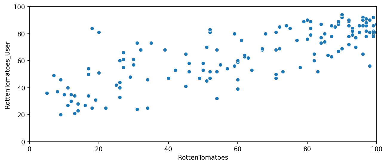
        Rotten Tamatoes 
        RT has two sets of reviews, their critics reviews (ratings published by official critics) and user reviews.
        
plt.figure(figsize=(10,4),dpi=150)
sns.scatterplot(data=all_sites,x='RottenTomatoes',y='RottenTomatoes_User')
plt.xlim(0,100)
plt.ylim(0,100)    

        Output
        

            
 

 
    
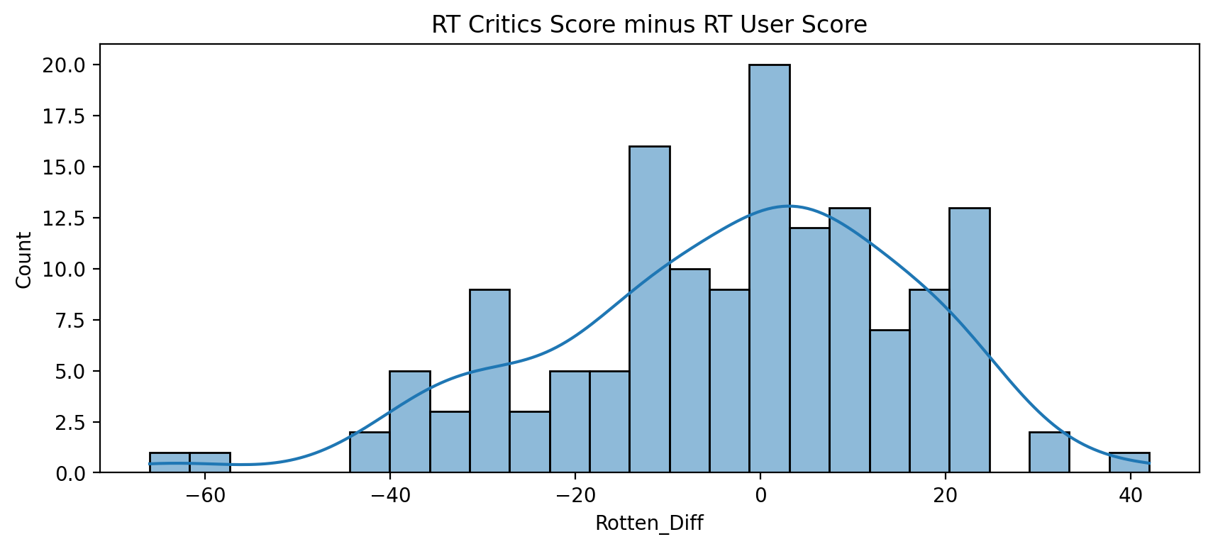
     Creating a new column based off the difference between critics ratings and users ratings for Rotten Tomatoes. ie :RottenTomatoes-RottenTomatoes_User
    
all_sites['Rotten_Diff']  = all_sites['RottenTomatoes'] - all_sites['RottenTomatoes_User']


    Output
    





    
    the Mean Absolute Difference between RT scores and RT User scores is.
    
all_sites['Rotten_Diff'].apply(abs).mean()

    Output
    
        15.095890410958905
                





    
    Histogramsof distribution of the differences between RT Critics Score and RT User Score.
    
plt.figure(figsize=(10,4),dpi=200)
sns.histplot(data=all_sites,x='Rotten_Diff',kde=True,bins=25)
plt.title("RT Critics Score minus RT User Score");

    Output
    

                





    
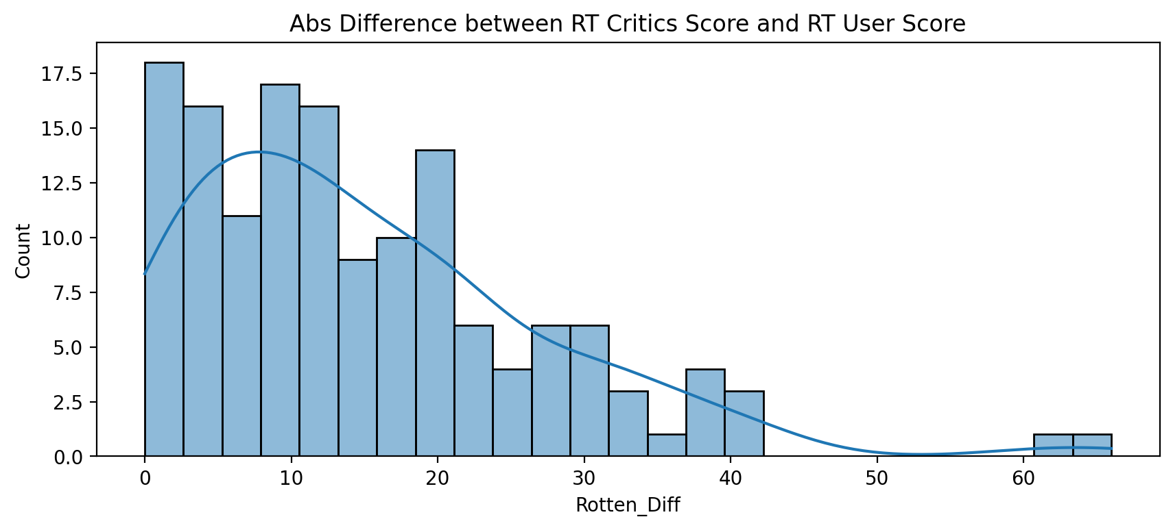
     distribution of the absolute value difference between Critics and Users on Rotten Tomatoes.
    
plt.figure(figsize=(10,4),dpi=200)
sns.histplot(x=all_sites['Rotten_Diff'].apply(abs),bins=25,kde=True)
plt.title("Abs Difference between RT Critics Score and RT User Score");
    Output
    
        
                





    
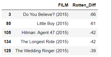
     the top 5 movies, users rated higher than critics on average
    

all_sites.nsmallest(5,'Rotten_Diff')[['FILM','Rotten_Diff']]

    Output
    
        
                



    
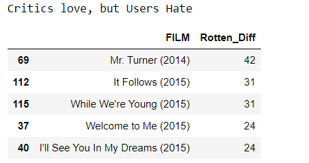
    the top 5 movies critics scores higher than users on average.
    
print("Critics love, but Users Hate")
all_sites.nlargest(5,'Rotten_Diff')[['FILM','Rotten_Diff']]

    Output
    
        
                



    MetaCritic
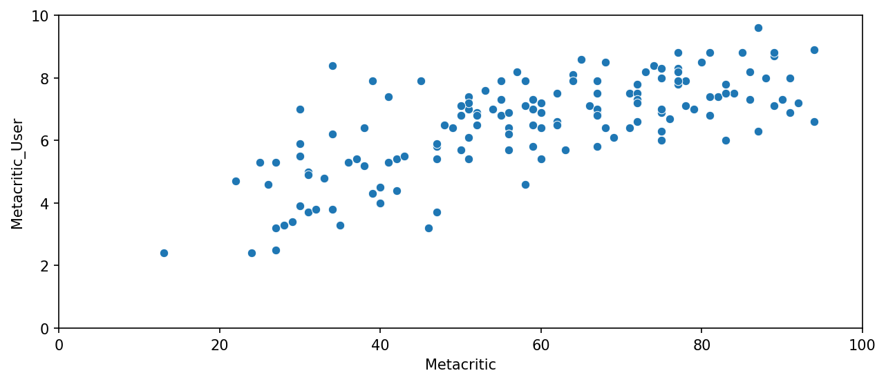
    a scatterplot of the Metacritic Rating versus the Metacritic User rating.
    
plt.figure(figsize=(10,4),dpi=150)
sns.scatterplot(data=all_sites,x='Metacritic',y='Metacritic_User')
plt.xlim(0,100)
plt.ylim(0,10)

    Output
    

                



    
    the highest Metacritic User Vote count for a movie
    
all_sites.nlargest(1,'Metacritic_user_vote_count')

    Output
    
        
                




    IMBD
    a scatterplot for the relationship between vote counts on MetaCritic versus vote counts on IMDB.
    
plt.figure(figsize=(10,4),dpi=150)
sns.scatterplot(data=all_sites,x='Metacritic_user_vote_count',y='IMDB_user_vote_count')

    Output
    

                


    
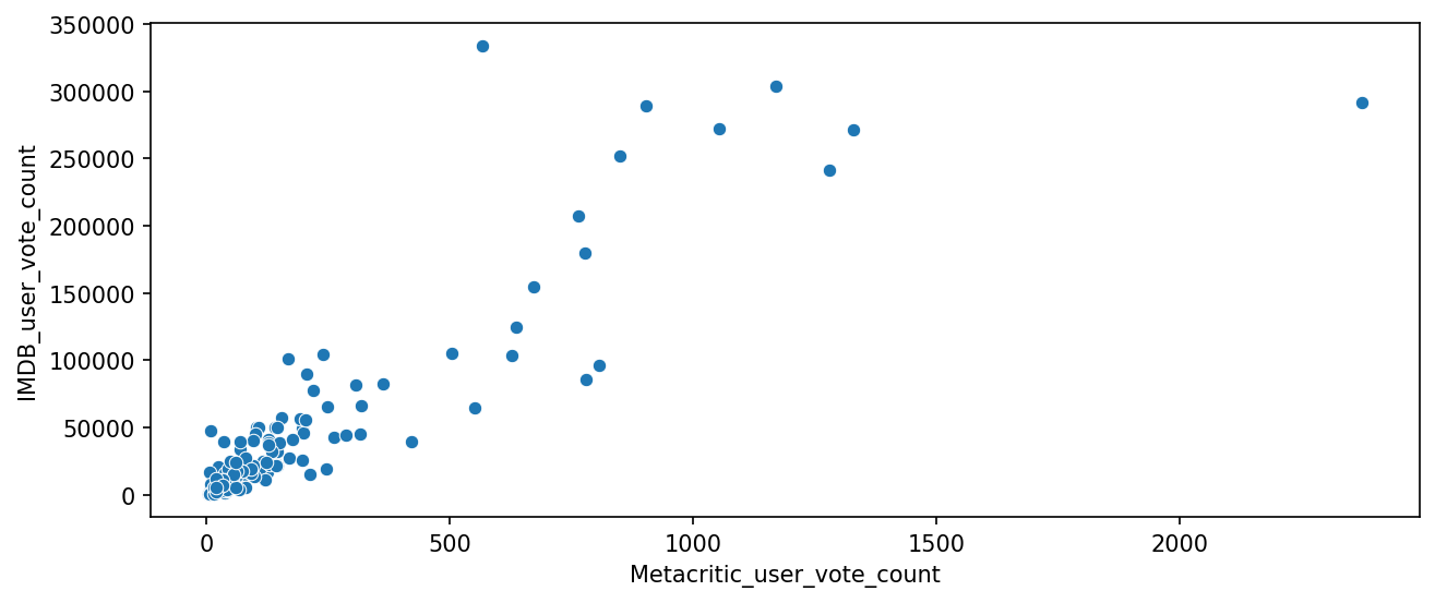
    the highest IMDB user vote count for a movie
    
all_sites.nlargest(1,'IMDB_user_vote_count')

    Output
    
        
                




     

     Part 3: Fandago Scores vs. All Sites 
    
        
         Combining the Fandango Table with the All Sites table, by inner merge to merge together both DataFrames based on the FILM columns.
        
df = pd.merge(fandango,all_sites,on='FILM',how='inner')


        Output
        
            
            
        

        
            
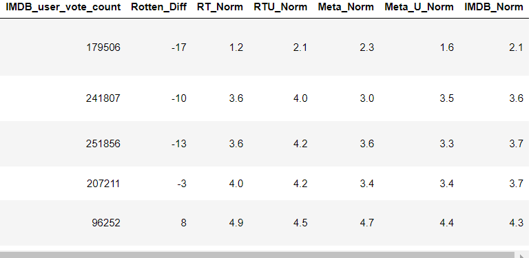
             Creating new normalized columns for all ratings so they match up within the 0-5 star range shown on Fandango.
            
df['RT_Norm'] = np.round(df['RottenTomatoes']/20,1)
df['RTU_Norm'] =  np.round(df['RottenTomatoes_User']/20,1)
df['Meta_Norm'] =  np.round(df['Metacritic']/20,1)
df['Meta_U_Norm'] =  np.round(df['Metacritic_User']/2,1)
df['IMDB_Norm'] = np.round(df['IMDB']/2,1)              
                df.head()
    
            Output
            

                
            



            
                
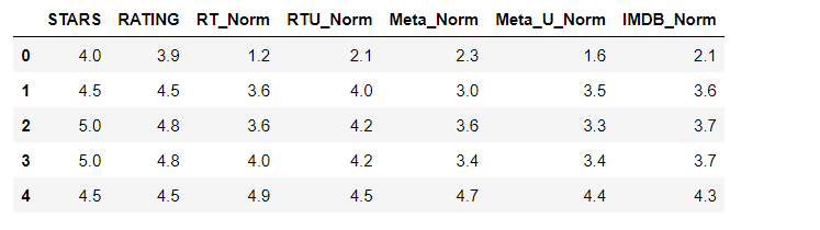
                 Now creating a norm_scores DataFrame that only contains the normalizes ratings. Include both STARS and RATING from the original Fandango table
                
norm_scores = df[['STARS','RATING','RT_Norm','RTU_Norm','Meta_Norm','Meta_U_Norm','IMDB_Norm']]
norm_scores.head()
        
                Output
                
                    
                    
                




                
                    
                    Comparing Distribution of Scores Across Sites
                    
def move_legend(ax, new_loc, **kws):
old_legend = ax.legend_
handles = old_legend.legendHandles
labels = [t.get_text() for t in old_legend.get_texts()]
title = old_legend.get_title().get_text()
ax.legend(handles, labels, loc=new_loc, title=title, **kws)
fig, ax = plt.subplots(figsize=(15,6),dpi=150)
sns.kdeplot(data=norm_scores,clip=[0,5],shade=True,palette='Set1',ax=ax)
move_legend(ax, "upper left")
            
                    Output
                    

                        
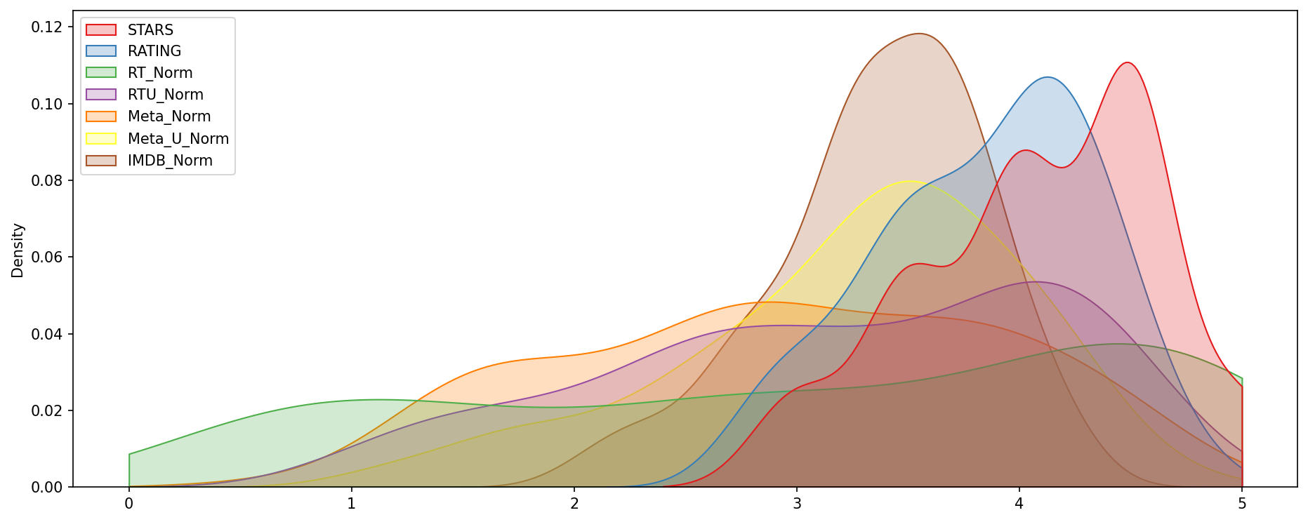
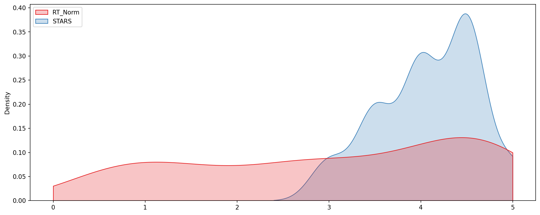
                        Clearly Fandango has an uneven distribution. We can also see that RT critics have the most uniform distribution. Let's directly compare these two
                    



                    
                        
                         A KDE plot that compare the distribution of RT critic ratings against the STARS displayed by Fandango.
                        
fig, ax = plt.subplots(figsize=(15,6),dpi=150)
sns.kdeplot(data=norm_scores[['RT_Norm','STARS']],clip=[0,5],shade=True,palette='Set1',ax=ax)
move_legend(ax, "upper left")
                
                        Output
                        

                            
                        

                        
                            
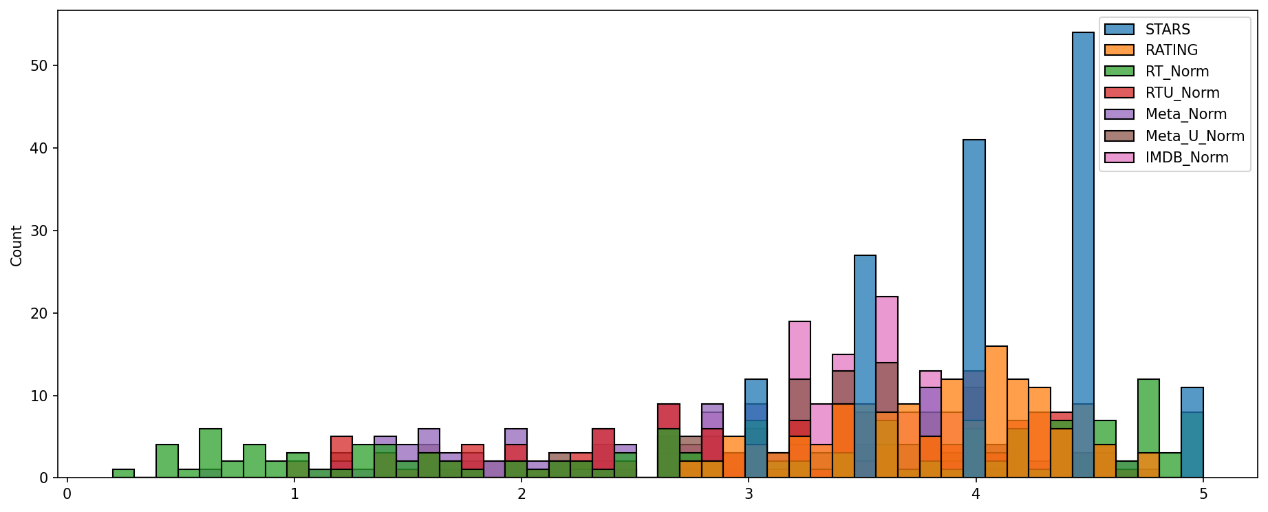
                            histplot which is  comparing all normalized scores.
                            
plt.subplots(figsize=(15,6),dpi=150)
sns.histplot(norm_scores,bins=50)
                    
                    
                            Output
                            

                                
                            

                            
                                
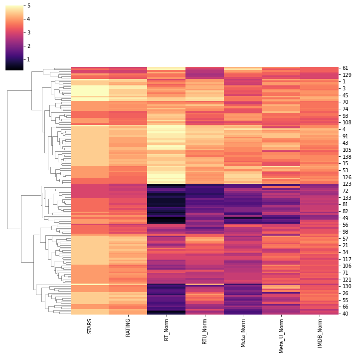
                                the worst movies rated across all platforms.
                                
sns.clustermap(norm_scores,cmap='magma',col_cluster=False)
                        
                        
                                Output
                                

                                    
                                


   
                                
                                    
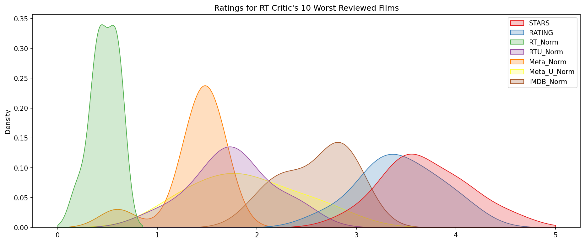
                                    The distribution of ratings across all sites for the top 10 worst movies.
                                    
plt.figure(figsize=(15,6),dpi=150)
worst_films = norm_films.nsmallest(10,'RT_Norm').drop('FILM',axis=1)
sns.kdeplot(data=worst_films,clip=[0,5],shade=True,palette='Set1')
plt.title("Ratings for RT Critic's 10 Worst Reviewed Films");
                            
                                    Output
                                    
                        
                                        
                                    


                                

                                
                                    Conclusion 
                                     Clearly Fandango is rating movies much higher than other sites, especially considering that it is then displaying a rounded up version of the rating. the top 10 worst movies, based off the Rotten Tomatoes Critic Ratings are :
                                    
norm_films = df[['STARS','RATING','RT_Norm','RTU_Norm','Meta_Norm','Meta_U_Norm','IMDB_Norm','FILM']]
norm_films.nsmallest(10,'RT_Norm')                           
                            
                                    Output
                                    

                                        
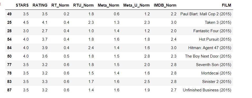
                                        Here we can clearly see tekken film  got 4.5 stars from fandango, on the other hand comparison to Rotten tamatoes which had gave 0.4 rating  
                                    

                                 
            

                                        
                                            
                                            
                                            
norm_films.iloc[25]                                    
                                    
                                            Output
                                            
            
                                                
                                            


                                            
                                        
                                            
                                            
                                            
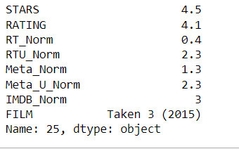
result = 0.4+2.3+1.3+2.3+3
avg_review =  result/5                                      
                                    
                                            
                                            
avg_review = 1.86 

                                             

 Hence Fandango is showing around 3-4 star ratings for films 
    that are clearly bad! Notice the biggest offender, 
    Taken 3!. Fandango is displaying 4.5 stars on their 
    site for a film with an average rating of 1.86 across 
    the other platforms!

Fandango

Aim

Technologies Used

Data

all_sites_scores.csv

fandango_scape.csv

part 1 :Fandango site

Output

Output

Output

Output

Output

Output

Output

Output

Output

Output

Part 2: Comparison of Fandango Ratings to Other Sites

Output

Output

Rotten Tamatoes

Output

Output

Output

Output

Output

Output

Output

MetaCritic

Output

Output

IMBD

Output

Output

Part 3: Fandago Scores vs. All Sites

Output

Output

Output

Output

Output

Output

Output

Output

Conclusion

Output

Here we can clearly see tekken film got 4.5 stars from fandango, on the other hand comparison to Rotten tamatoes which had gave 0.4 rating

Output

avg_review = 1.86

Hence Fandango is showing around 3-4 star ratings for films that are clearly bad! Notice the biggest offender, Taken 3!. Fandango is displaying 4.5 stars on their site for a film with an average rating of 1.86 across the other platforms!